Looking to enhance your audio production skills? Consider reinforcing your “major” with a dash of Electronics 101. The oscilloscope is the most important tool in the “Tech’s Files” arsenal. Geek instinct and plenty of e-mails tell me that too many people are experimenting in the dark. A 20MHz dual-trace oscilloscope is all you need for most analog audio work and is available new for less than $500. Hopefully, this article will inspire you to buy a ‘scope and we can zoom into more waves in the coming year.
An oscilloscope converts electrical signals into visual images known as waveforms. A traditional analog ‘scope uses a Cathode Ray Tube (CRT) for this purpose. (While an LCD enables portability, the smaller/cheaper versions tend to have “digitized” artifacts that, for the inexperienced, make it hard to judge signal quality.) A CRT is like a television’s picture tube: High voltage accelerates streams of electrons to bombard a phosphor-coated screen, creating a visible light beam in the process. The beam is deflected up, down and across the screen by electrostatic force. It’s amazingly simple and remarkably precise. A TV CRT, on the other hand, requires electromagnetic force: four amplifier-driven coils — two for horizontal, two for vertical.
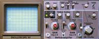
Figure 1: a dual-trace oscilloscope with a blank screen
There are many different types of ‘scopes, from the no-frills analog example used in Fig. 1 to digital versions with memory for image and data storage. Readers who want to modify or upgrade their gear should be willing to invest a little money in test equipment. Why? Because, for example, a circuit oscillating outside the range of human hearing can be deadly to tweeters. A ‘scope can reveal the danger before any damage is done.
Figure 2: an oscilloscope display with a composite image of
various waveforms (a simulation that is not possible in the real world). In green at top, the Lissajous patterns are the result of
X-Y phase measurements. In blue, a square wave (far-left) as manipulated by equalization (or bad capacitors) to the right. At bottom, a sine wave (green) and two versions of distortion (violet and red).
MODES
An oscilloscope has two basic modes: X-Y and Sweep, with the former used to measure the phase differences between two channels, and the latter to display amplitude vs. frequency. In X-Y mode, a sine wave connected to either the vertical or horizontal input will create a vertical or horizontal line, respectively. A mono signal connected to both channels generates a 45-degree diagonal line (Fig. 2, top row, left). If the polarity of either channel is flipped 180 degrees, then the line changes direction (Fig. 2, top row, right). In between are some of the Lissajous pattern variations representing 45- and 90-degree phase shifts. It’s quite common to use a ‘scope (and now software) to monitor a stereo signal in X-Y mode.
Figure 3: an oscilloscope’s vertical amplifier section
VERTIGO
A dual-trace ‘scope has two vertical inputs (Fig. 3): Input A becomes the vertical channel, and in X-Y mode, input B is routed to the horizontal channel. Note: In this example, three switches must be flipped for the ‘scope to be in X-Y mode: two in the trigger section (Fig. 5) and one in the vertical amplifier.
Figure 4: the horizontal sweep section of a ’scope
SWEEP
In Sweep mode, a sawtooth oscillator driving the horizontal amplifier (Fig. 4) moves the beam from left to right. Most of the time, the sweep rate is so fast that the beam appears to be a line (aka the trace). When the sweep rate is slow enough, you’ll see a spot move across the screen. Faster sweep rates reduce the brightness of the trace, something to consider when making a purchase if you plan to do RF work, for example. Better, more expensive ‘scopes have more consistent brightness throughout the sweep’s range.
The display screen has a graticule comprising horizontal and vertical lines that are typically one centimeter apart. Both axes display volts per division when in X-Y mode. In Sweep mode, the horizontal axis now indicates time per division. Measuring amplitude is pretty straightforward, but translating waveforms into frequency requires some ciphering. A single sine wave that precisely fills the screen (bottom example in Fig. 2) is 10 cm wide. If the sweep rate is 0.1 ms/div, then the total sweep time for that wave is 1 ms (0.001 seconds), and one over that amount will reveal the number of cycles per second; in this case, 1,000 Hertz, or 1 kHz.
Figure 5: The trigger section of an oscilloscope stabilizes the image much like a noise gate so that the waveform starts where you want it—at the positive or negative excursion or at the zero crossing.
ROY ROGERS’ HORSE
An oscilloscope also has a trigger section to stabilize the waveform (Fig. 5). In Auto mode, the trace is always visible, with or without a signal connected to the vertical input. Normal mode is similar to a noise gate: The trace is turned on once the amplitude reaches threshold.
The range and effectiveness of the controls are most obvious when viewing a sine wave. The Trigger Level control determines where the sine wave starts at, plus or minus the zero crossing. A Trigger Slope switch is also provided so that sine will start on its positive or negative slope. The Trigger can be optimized to expect high- or low-frequency signals from either A or B inputs, the power line (good for power supply tests) or an external source.
A square wave is essentially on or off, so either the positive or negative half of the wave will appear first. Square waves with superfast rise times will have almost no visible vertical traces, minimizing the effect of the Trigger Level control. Don’t worry, it’s not broken.
COMPENSATION
The high input impedance of the vertical amplifier specified in this example is 1 megohm with 25 picofarads in parallel — great for not loading a signal, but it also makes the ‘scope cable-sensitive. Consider that high-quality cable has 17pF/foot capacitance and the total (cable plus input capacitance) could easily reach 100 pF. This could potentially load high-impedance, high-frequency circuits. For this reason, most ‘scope probes feature a 10X mode that inserts a 10-megohm resistor to further increase the input impedance. While this reduces the signal by one-tenth, when combined with an adjustable parallel capacitor, the probe can be “compensated” for cable loss.
A fixed-frequency square wave oscillator is provided on the front panel for probe calibration, both amplitude and frequency response. It’s labeled CAL and is centered at the bottom of the vertical amplifier (Fig. 3). Of the four square waves on the display (Fig. 2), the one at the far-right is an example of an under-compensated probe. (High frequencies are rolled off.) The example just to the left is overcompensated. (High frequencies are boosted.) Of course, we want a perfectly square wave (far left).
SUM DIFFERENCE
I’ve had an oscilloscope since my sophomore year of high school. Reflections on my early “eureka” moments, plus tips for geeks in training, will be online at www.tangible-technology.com, with an extended version of this column and summaries of additional pieces of test equipment.
Eddie applied for a teaching position near the Twin Cities. By the time you read this, he may be deeply involved in the fall semester.